UFO Sightings

Want to smash together 10 different data files in R? Got untidy dates in need of formatting? Here’s an extreme¹ example of data cleaning several data sets.

I’m not sure about extraterrestrial life. But while performing data analysis here on Earth, we seldom receive clean data in one single file. We’ll learn more about the tidyverse by exploring the universe of variables we could possibly connote with UFO sightings.

Step 0: Read in libraries

First, let’s load the necessary packages or libraries. If you don’t have any one of the packages installed, try typing the command below into your Console. Say you don’t have the tidyverse package installed:

install.packages("tidyverse")

Now we’re ready to load those libraries!

library(here)
library(tidyverse)
library(data.table)
library(janitor)
library(noncensus)
library(zoo)
library(plyr)
library(datetime)

library(purrr)
library(lmtest)
library(ggplot2)
library(ggrepel)
library(GGally)
library(lubridate)

Step 2: Download files

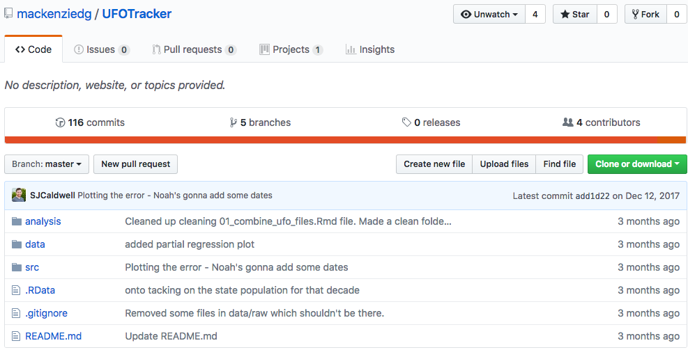
Let’s download the files from this Github repo. If you’re not as comfortable with Git, you can just click the green button Clone or download in the upper right corner and download zip.

Step 3: Read in files

I used to write file.path() to set relative paths to files, but recently I discovered the here package through Jenny Bryan.

@krlmlr The `here` package is bringing me such happy today ☺️ https://t.co/is1rOjy3XN (@STAT545 students already asking about subdirs ...)

— Jenny Bryan (@JennyBryan) September 16, 2016

Blog post elaborating on my advice to avoid setwd() and rm(list = ls()) at top of an #rstats script.
Wow that really touched a nerve 😮https://t.co/YDvVUQOMKx https://t.co/b4SpNhBYUX

— Jenny Bryan (@JennyBryan) December 12, 2017

The here() function helps ensure consistency of file paths–even when we have nested files.

beer.path <- here("raw", "brew_count_by_state_1984_2017.csv")
movies.path <- here("raw", "alien_movies_per_year.csv")
gdp.path<- here("raw", "gdp_per_capita_per_year.csv"
internet.path <- here("raw", "internet.csv"
internet.rurality.path <- here("raw", "internet_by_rurality.csv"
usafbase.path <- here("raw", "usaf_base_locs.csv"
statepops.path <- here("raw", "state_pops.csv"
sightings.path <- here("raw", "ufo_sightings.csv"
allmovies.path <- here("raw", "number_of_movies_per_year.csv"
statepops3.path <- here("raw", "statepops.db3.csv")

Now we’re ready to read the csv files. I used to use read.csv but I started using fread from the data.table package more often since it’s significantly faster for larger data sets. (You can learn more about fread and other ways of reading data into R through Datacamp).

The na.strings parameter automatically converts specific strings into NA. This is useful since different files will have different entries for NA. For example: the beer.csv file contains a bunch of null entries that are denoted as asterisks * or empty strings " " while the sightings.csv file will contain null entries denoted as an empty string, "unknown", or "--".

beer.raw <- fread(beer.path, header=TRUE, na.strings=c("*", ""))
sightings.raw <- fread(sightings.path, header = TRUE, na.strings = c("", "Unknown", "--"))
movies.raw <- fread(movies.path, header = TRUE)
gdp.raw <- fread(gdp.path, header = TRUE)
internet.raw <- fread(internet.path, header = TRUE)
internet.rurality.raw <- fread(internet.rurality.path, header = TRUE)
usafbase.raw <- fread(usafbase.path, header = TRUE, na.strings = c(""))
statepops.raw <- fread(statepops.path, header = TRUE)
allmovies.raw <- fread(allmovies.path, header = TRUE)
statepops3.raw <- fread(statepops3.path, header = TRUE)

Step 4: Data cleaning

Now that we’ve read in our data sets, we’re ready to start cleaning up each individual data set. First, let’s start with the breweries data.

Step 4a: Tidy Beers

In the quest for consistency, the rename function from the dplyr library allows us to easily rename variables. Here we are renaming STATE as state and assigning this change to a new dataframe called beer.db. This helps us distinguish the raw dataframes we read in from the cleaned dataframes we desire in the end.

beer.db <- beer.raw %>% 
  rename(state = STATE)

Now let’s get rid of a bunch of unwanted text in the file. At the bottom of the state column, there’s a bunch of text we don’t need. We can filter out rows in the state column that are NA’s, text like “Total” or “Other” or etc.

beer.db <- beer.db %>% 
  filter(! (is.na(state) | state == "Total" | state == "Other" |
              state == "* No reportable data" | 
              state == "«This list will be updated quarterly."))

It would be cumbersome to keep reassigning the beer.db dataframe every time we wanted to make a change. Fortunately the pipe operator %>% allows us to chain together all these manipulations to the beer.raw dataframe and assign it to a variable called beer.db in one tidy sweep.

beer.db <- beer.raw %>% 
  dplyr::rename(state = STATE) %>%
  filter(! (is.na(state) | state == "Total" | state == "Other" |
              state == "* No reportable data" | 
              state == "«This list will be updated quarterly.")) %>%
  mutate(state = as.factor(state)) %>%
  gather_("year", "breweries", as.character(seq(1984, 2017))) %>%
  mutate(breweries = as.numeric(breweries)) %>%
  filter(1984 <= year & year <= 2016) %>%
  mutate(year = as.numeric(year))

Step 4b: Tidy the Internets

# Combine the two into one data frame based on year
internet.db <- merge(internet.raw, internet.rurality.raw, by = "Year")

# Rename the columns
colnames(internet.db) <- c("year", "internet_avg", "internet_urban", "internet_suburban", "internet_rural")

Step 5: Group the states into regions.

The states data set from the noncenusus package comes in handy since we want to bin each state into a region category. For example: California will be considered “west” and Massachusetts will be considered “east.”

data(states)

statepops.db <- statepops.raw %>% 
  #gather_("Name", "year", "population")
  gather_("year", "population", as.character(seq(1960,2010,10))) %>% 
  filter(Name %in% state.name) %>% 
  mutate(year = as.integer(year)) %>% 
  mutate(population = as.numeric(gsub(",", "", population)))

Let’s filter for just the names of states.

statepops.db2 <- statepops.raw %>% 
  filter(Name %in% state.name)  

statepops.db3 <- data.frame(t(statepops.db2))

We will only keep data from years 1970 to 2016 since the timeframe coincides with the rest of our data sets. Let’s write the clean data to a csv file within the /clean/ folder to tidy up a little.

yrs <- 1970:2016
yrs <- zoo(NA, datetime::as.year(yrs))
zpops <- zoo(select(statepops3.raw, -year), as.year(statepops3.raw$year))

z <- merge(yrs, zpops)
z <- z[, colnames(z) != "yrs"]
interps <- na.spline(z)
interps <- as.data.frame(interps)
interps$year <- rownames(interps)
colnames(interps) <- mapvalues(colnames(interps), state.name, state.abb)
interps <- interps %>%
    filter(year >= 1974)
fwrite(interps, "./clean/interpolated_pops.csv")

Tidy the UFO Sightings

If you’ve read this far must be wondering, “What do those two colons :: mean?!” Since different packages might share the same name for functions, this is how R differentiates them. For example: the filter function from dplyr package, which is not the same as filter from the stats package. To be frank, the code below doesn’t look most elegant but we get the job done.

sightings.db <- sightings.raw %>% 
  mutate(state = toupper(state)) %>% 
  mutate(year = as.numeric(format(as.Date(date_time, format="%m/%d/%y"),"%Y"))) %>% 
  dplyr::filter(state %in% state.abb) %>% 
  dplyr::filter(1974 <= year & year <= 2016) %>% 
  dplyr::count(year, state) %>% 
  dplyr::rename(num_sightings = n) %>%
  dplyr::left_join(states, by = c("state" = "state")) %>%
  dplyr::select(-area, -population, -division, -capital) %>%
  dplyr::mutate(decade = year - (year %% 10))

Step 6: Normalize the number of sightings by the population of each state

Perhaps the number of sightings is highly skewed by scale of population in each state. Let’s normalize the number of sightings per capita.

df$sightings_per_thousand <- (df$sightings / df$pop) * 1000

interps <- melt(interps)
interps$year <- as.numeric(interps$year)
sightings.db2 <- as.data.frame(sightings.db) %>% 
dplyr::left_join(interps, by=c("year"="year", "state"="variable")) %>%
dplyr::mutate(sightings_per_100k=((num_sightings/value) * 100000)) %>% 
dplyr::select(year, state, region, sightings_per_100k)

write_csv(sightings.db2, "./clean/sightings_db2.csv")

Using population data from the Census, we’re able to get a feel for the population of each state during each decade.

# statepops.raw$Name <- mapvalues(statepops.raw$Name, state.name, state.abb)
# state_pops <- statepops.raw %>%
#     filter(Name %in% state.abb) %>%
#     select(one_of(c("1970", "1980", "1990", "2000", "2010"))) %>%
#     apply(1, mean)

Step 7: Normalize Movies By Total Movies That Year

Also remember to stick within the time domain of our other data.

#all_movies <- allmovies.raw[nrow(allmovies.raw):1,]
allmovies.raw <- allmovies.raw %>% 
  filter(1974 <= year & year <= 2016)

Divide number of alien movies that year. Divide by total box office movies that came out that year.

The number is small, so interepretability may be an issue here. Careful!

movies.db <- movies.raw %>% 
  filter(1974 <= year & year <= 2016) %>%
  left_join(allmovies.raw, by=c("year"="year")) %>% 
  mutate(alienmovies_per_year = num_movies/total_movies) %>% 
  select(year, alienmovies_per_year)

gdp.db <- gdp.raw %>% 
  clean_names() %>% 
  dplyr::rename(year = year_and_category) %>% 
  filter(year >= 1974) %>% 
  select(year, per_capita_gdp_current)

The data on number of US air bases per state is a bit sparse, so be sure to handle missing entries.

usafbase.db <- usafbase.raw %>% 
  #filter(State == "FL") %>% 
  # rename(state = State) %>% 
  group_by(State) %>%
  dplyr::count() %>%
  merge(state.abb, by.x="State", by.y=1, all=T) %>%
  mutate(n=replace(n, is.na(n), 0)) %>%
  filter(!is.na(State)) %>% 
  dplyr::rename(afbase_per_state = n) %>% 
  dplyr::rename(state = State)

Step 8: Join files together

When you join two data sets, you join based on shared values of the rows. For example: I want to pair up all the entries from beer.db and movies.db based on year.

all.states.normalized.df <- sightings.db2 %>% 
    left_join(beer.db, by=c("year" = "year", "state"= "state")) %>% 
    left_join(movies.db, by = c("year" = "year")) %>% 
    left_join(gdp.db, by = c("year" = "year")) %>%
    left_join(internet.db, by=c("year" = "year")) %>% 
    left_join(usafbase.db, by=c("state" = "state")) %>%
    left_join(interps, by=c("year"="year", "state"="variable")) %>%
    dplyr::rename(population=value) %>%
    mutate(normalized_afb_count=afbase_per_state/population*1000000) %>%
    select(one_of("state", "year", "region", "sightings_per_100k", "alienmovies_per_year", "per_capita_gdp_current", "internet_avg", "internet_urban", "internet_suburban", "internet_rural", "normalized_afb_count"))

all.states.normalized.df[is.na(all.states.normalized.df)] = 0

We’re almost there!

Now let’s select the data between the year 1985 and 2014 inclusive.

all.states.normalized.df <- all.states.normalized.df %>%
    filter(year >= 1985 & year <= 2014)

Step 9: Write out

Finally we’re ready to write the clean data frame to a csv. We did it!

fwrite(all.states.normalized.df, "clean/all_states_normalized.csv")